Understanding Facebook’s Prophet: A Guide to Time Series Forecasting
Introduction to Prophet
In the realm of data analysis and forecasting, Facebook’s Prophet has emerged as a powerful tool, particularly for handling time series data. Developed by Facebook’s Core Data Science team, Prophet is an open-source library designed for making forecasts into the future. It is tailored specifically for business forecasts, but its flexibility allows it to be used for a wide range of time series forecasting tasks.
Key Features of Prophet
Prophet stands out due to its ability to handle the various challenges of time series forecasting, such as:
- Trend changes: It adapts to changes in trends by fitting non-linear trends with daily, weekly, and yearly seasonality.
- Holiday effects: Prophet can incorporate holidays and events that might affect the forecast.
- Missing data and outliers: It is robust to missing data and shifts in the trend, and can accommodate outliers.
How Prophet Works
Prophet employs an additive regression model comprising several components:
- Trend: Models non-periodic changes.
- Seasonality: Represents periodic changes (e.g., weekly, monthly, yearly).
- Holidays: Incorporates irregular events like Black Friday, Cyber Monday, etc.
- Additional regressors: Allows incorporating other variables to improve the forecast.
Applications of Prophet
Prophet’s versatility makes it applicable in various fields:
- Retail and Sales Forecasting: Predicting product demand, sales, and inventory requirements.
- Stock Market Analysis: Forecasting stock prices and market trends.
- Weather Forecasting: Predicting weather patterns and temperature changes.
- Resource Allocation: In organisations for planning and allocating resources based on forecasted demand.
Conclusion
Facebook’s Prophet has revolutionised time series forecasting by making it more accessible and adaptable to different scenarios. Whether you are a seasoned data scientist or a beginner, Prophet offers an intuitive and powerful tool for forecasting tasks.
Methods for Forecasting Response Time and Resource Requirements:
Time Series Forecasting (ARIMA, LSTM)
Data Processing:
- Time series forecasting models like ARIMA (Autoregressive Integrated Moving Average) and LSTM (Long Short-Term Memory) networks require the data to be in a time series format, where observations are ordered chronologically.
- For ARIMA, a key requirement is stationarity, meaning the statistical properties of the series (mean, variance) do not change over time. This often requires transforming the data, like differencing the series, to stabilize the mean.
- Seasonal decomposition can be used to separate out seasonal patterns and trends from the time series, which is particularly useful if the response times have seasonal variability.
- For LSTM, a type of recurrent neural network, the data should not only be in chronological order but also might need to be reshaped or transformed into specific formats (like 3D array structures) suitable for LSTM’s input requirements.
Use Case:
- ARIMA is well-suited for datasets where historical data shows clear trends or patterns over time, and where these patterns are expected to continue.
- LSTM is ideal for more complex scenarios where the relationship between past and future points is not just linear or seasonal but might involve deeper patterns that standard time series models can’t capture.
Support Vector Machines (SVM)
Data Processing:
- SVMs require all inputs to be numerical. Categorical data, such as incident types or districts, must be converted into numerical form through techniques like one-hot encoding.
- Feature scaling is crucial for SVMs as they are sensitive to the scale of the input features. Standardization (scaling features to have a mean of 0 and a variance of 1) is a common approach.
- It’s also important to identify and handle outliers, as SVMs can be sensitive to them, especially in cases where kernel functions are used.
Use Case:
- SVMs are effective when the dataset has a high number of features (high-dimensional space) and when the classes are separable with a clear margin.
- They are well-suited for scenarios where the response times or resource requirements show a clear distinction or pattern based on the incident features.
Neural Networks
Data Processing:
- Similar to SVMs, neural networks require numerical inputs. Categorical variables should be encoded.
- Feature scaling, such as min-max normalization or standardization, is essential as it helps in speeding up the learning process and avoiding issues with the convergence of the model.
- Depending on the size and complexity of the dataset, the data might need to be batched, i.e., divided into smaller subsets for efficient training.
Use Case:
- Neural networks are particularly effective for complex and large datasets where the relationships between variables are not easily captured by traditional statistical methods.
- They are suitable for scenarios where the response times or resource requirements are influenced by a complex interplay of factors, and where large amounts of historical data are available for training.
Application in Forecasting Response Time and Resource Requirements
- Time Series Forecasting: Use ARIMA or LSTM to model and predict response times based on historical trends. This approach can capture patterns over time, including seasonality and other time-related factors.
- SVM: Apply SVM to classify incidents into categories based on their likely response time or resource requirements. This method can be useful in scenarios where incident attributes clearly define the response or resource needs.
- Neural Networks: Employ neural networks for more complex prediction tasks, such as when the response time is influenced by a wide array of factors, including non-linear and non-obvious relationships in the data.
In each case, the model should be trained on historical data and validated using techniques like cross-validation to ensure its reliability and accuracy. The choice of model will depend on the specific characteristics of the data and the nature of the forecasting task at hand.
Predictive Model for Incident Frequency
Initial Introduction- Primary Data Analysis of Fire Incidents Dataset
Incident Description Analysis Results
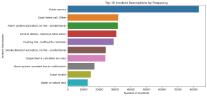
The bar graph illustrates the top 10 incident descriptions by frequency. The most common description is ‘Public service’, followed by ‘Good intent call, Other’, ‘Alarm system activation, no fire – unintentional’, and others. This visualization helps identify which types of incidents are most frequently encountered, which is vital for predictive modeling in terms of incident frequency and types.
Understanding the prevalence of these incident descriptions is key to formulating predictive models that can anticipate the likelihood of different incidents occurring, aligning with the project’s aim to predict incident frequencies and types.
Temporal Analysis Results
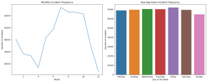
Monthly Incident Frequency: The line graph shows the number of incidents by month. There’s a noticeable seasonal trend, with incident frequencies peaking in the summer months (June, July, August). This pattern suggests that certain times of the year may have a higher likelihood of incidents, which is crucial for time series forecasting and predictive modeling.
Daily Incident Frequency: The bar graph illustrates the average number of incidents per day of the week. The data indicates a fairly consistent frequency throughout the week, with a slight increase on Fridays. This insight is important for understanding daily trends in incident occurrences.
This temporal analysis supports the project’s objective of identifying seasonal and daily patterns in emergency incidents. It lays the groundwork for developing forecasting models that can predict incident frequencies based on time variables.
Response Time Analysis Results Based on Incident Description
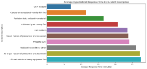
The bar graph presents the average hypothetical response times for the top 10 incident descriptions. The response times vary considerably across different types of incidents, indicating that some emergencies may generally require longer response times. For instance, incidents like ‘CISM Incident’ and ‘Camper or recreational vehicle (RV) fire’ show different average response times.
While this data is hypothetical, in a real-world scenario, analyzing actual response times would be vital for predicting the time required to respond to various emergencies. This aligns with focusing on forecasting response times and resource requirements based on incident descriptions.
This analysis, using a hypothetical model, demonstrates the potential of applying real response time data in machine learning models. Such models can be used to forecast response times and resource requirements for different incidents based on their descriptions, enhancing the efficiency and effectiveness of emergency response services.
Overall, these analyses provide a comprehensive understanding of the dataset’s potential for addressing the questions in the previous post. They highlight how machine learning and time series forecasting can be applied to predict incident frequencies, descriptions, and response requirements, key for effective emergency management and planning
Fire Incidents Dataset. What are we predicting?
Predicting Incident Frequency and Types
One significant question that can be addressed using machine learning is predicting the frequency and types of incidents. By analyzing historical data, machine learning models can identify patterns and predict future occurrences of various incident types. This could involve questions like, “Which types of incidents are most likely to occur in a given district?” or “Is there a seasonal pattern to certain types of emergencies?” Such predictions can help emergency services in preemptive planning and resource allocation, ensuring readiness for specific types of incidents at different times of the year.
Forecasting Response Time and Resource Requirements
Machine learning can also be utilized to forecast response times and resource requirements for different incidents. By analyzing past data, predictive models can answer questions such as, “How long does it typically take for emergency services to respond to a certain type of incident in a specific area?” or “What resources are often required for different incident types?” This analysis can help in optimizing response strategies and ensuring that adequate resources are available and efficiently deployed, thereby potentially reducing response times and improving overall emergency service efficiency.
Understanding and Mitigating Financial Impacts
Finally, using time series forecasting, this dataset can provide insights into the financial impact of incidents over time. Questions like, “What is the projected financial impact of certain types of incidents in the future?” or “How does the financial impact of incidents vary throughout the year?” can be addressed. This information is crucial for budget planning for city councils, emergency services, and insurance companies. By understanding and predicting these financial impacts, stakeholders can better allocate funds, prepare for high-cost periods, and develop strategies to mitigate losses.
What is my chosen dataset and why?
I have chosen the Fire incidents dataset and the url for the download is https://data.boston.gov/dataset/ac9e373a-1303-4563-b28e-2.
The dataset comprising detailed incident reports offers a rich and impactful foundation for a data science project. Its relevance stems from the broad spectrum of real-world incidents it covers, ranging from emergency responses to property damage. This diversity not only allows for a comprehensive understanding of various emergency situations but also presents an opportunity to make a tangible impact. By analyzing this data, we can potentially enhance public safety, optimize response strategies, and improve resource allocation. The dataset’s detailed categorization of incidents, along with temporal data (date and time), geographical information (districts and street addresses), and estimated losses, provides a multifaceted view of emergency situations, making it an ideal candidate for in-depth data science exploration.
The rich and varied nature of this dataset opens up numerous possibilities for applying machine learning techniques. For instance, classification algorithms can be used to predict the type of incident based on the given input parameters, aiding in quicker and more accurate dispatch of emergency services. Furthermore, machine learning models can identify patterns and correlations within the data that are not immediately apparent, such as the relationship between incident types and geographical locations or times of day. This insight can guide emergency response units in strategic planning and preparedness. Additionally, anomaly detection algorithms can identify outliers in the data, which could signify unusual or particularly hazardous incidents, thus ensuring that such cases receive immediate attention.
The temporal aspect of this dataset makes it particularly suitable for time series analysis and forecasting. By employing time series forecasting models, we can predict future trends in incident occurrences, helping emergency services to prepare for periods of high demand. This aspect is crucial for efficient resource management, such as allocating personnel and equipment. Seasonal trend analysis can also reveal critical insights, such as identifying times of the year when certain types of incidents are more prevalent. This foresight can be instrumental in proactive planning, training, and public awareness campaigns. Moreover, the ability to forecast potential increases in certain types of incidents could also aid in budget planning and allocation for city councils and public safety organizations.
Exploring New Dimensions in Time Series Forecasting: Predictive Insights from Police Analysis Data
Case Study: Police Analysis Data
Let’s consider a hypothetical case study of police analysis data. This data isn’t just about the count of incidents. It encompasses various metrics such as the type of incidents, geographical locations, time of the day, response times, and outcomes. By applying time series forecasting to these different values, we can predict several aspects
The analysis of the police shooting data in the PDF provided offers some interesting insights from a time series perspective. Here’s a summary of the results:
- Data Collection: The data includes 8,002 shooting dates and 2,702 unique dates, reflecting police shooting incidents. This data was then used to count the number of shootings that occurred on each unique date.
- Initial Observations: The initial analysis involved plotting the sequence of counts (number of shootings per day). This provided a basic understanding of how the frequency of these incidents varied over time.
- Monthly Analysis: To gain a broader perspective, the daily counts were replaced with monthly counts. This step helped in visualizing longer-term trends and patterns in the data.
- Stationarity Test: A key part of time series analysis is determining if the data is stationary, meaning its statistical properties like mean and variance are constant over time. The document details the use of a unit root test, which indicated that the original time series data was likely not stationary. However, after differencing the data (calculating the difference between consecutive data points), the resulting series appeared to be stationary.
- Model Fitting: The analysis applied Mathematica’s TimeSeriesModelFit function, fitting an autoregressive moving-average (ARMA) model to the differenced data. This model helps in understanding the underlying patterns and can be used for forecasting.
- Predictions and Forecasting: The primary goal of time series analysis is to forecast future values. The document does not explicitly mention specific forecasts or predictions made from this data, but the methodologies and models applied are typically used to predict future trends based on historical data.
The analysis demonstrates the application of time series forecasting methods to a real-world dataset, highlighting the importance of checking for stationarity, transforming data accordingly, and fitting appropriate models for analysis and forecasting.
Understanding Time Series Forecasting: A Dive into Predictive Analysis
In the realm of data analysis, time series forecasting emerges as a critical tool for predicting future events based on past patterns. But what exactly is time series forecasting, and what type of data is ideal for leveraging its potential? Let’s explore.
What is Time Series Forecasting?
Time series forecasting involves analysing a collection of data points recorded over time, known as a time series, to predict future values. This approach is fundamental in various fields, from economics to environmental science, enabling experts to anticipate trends, seasonal effects, and even irregular patterns in future data.
A time series is essentially a sequence of data points indexed in time order, often with equal intervals between them. This could be anything from daily temperatures to monthly sales figures.
Ideal Data for Time Series Forecasting
The effectiveness of time series forecasting hinges on the nature of the data at hand. The ideal data should have these characteristics:
- Time-dependent: The data should inherently depend on time, showing significant variations at different time points.
- Consistent frequency: The data points should be recorded at regular intervals – be it hourly, daily, monthly, or annually.
- Sufficient historical data: A substantial amount of historical data is crucial to discern patterns and trends.
- Clear Trends or Seasonality: Data that exhibits trends (upward or downward movement over time) or seasonality (regular and predictable patterns within a specific time frame) are particularly suited for time series analysis.
- Stationarity (or transformed to be so): Ideally, the statistical properties of the series – mean, variance, and autocorrelation – should be constant over time. If not naturally stationary, data can often be transformed to achieve this property, enhancing the forecasting accuracy.
Real-World Application Example
One compelling example is the analysis of police shooting data. This data, indexed by the date of occurrence, exhibits time-dependent characteristics, making it suitable for time series analysis. By analysing the count of such events over time, patterns can be observed and used for forecasting future occurrences.
Conclusion
Time series forecasting stands out as a pivotal technique in data analysis, offering a window into future trends and patterns. Ideal time series data is time-dependent, consistently recorded, and exhibits trends or seasonality.