Month: October 2023

Introduction:
In an era where societal issues are under intense scrutiny, understanding the demographics of those affected by police shootings is paramount. This analysis provides a granular look into the interplay of age, race, and gender in police shootings, revealing some critical patterns and implications.

Breakdown by Age and Race:
When examining the age distribution across races:
Black Individuals: The median age was 31, with males having a right-skewed distribution around the late 20s and females around the early 30s.
Hispanic Individuals: The median age was 32 for males and 30 for females, both showing a right-skewed distribution.
White Individuals: Males had a median age of 38, while females had a median age of 39, both with a slightly right-skewed distribution.
Asian Individuals: Males had a median age of 34, while the smaller female sample had a median age of 47.

Breakdown by Race and Gender:
Males overwhelmingly dominate the dataset across all racial categories, accounting for about 95% of the total. However,
White and Black Categories: Both races had relatively higher female representations, with females accounting for approximately 5% of the total in these categories.
Other Racial Categories: Female representation was significantly smaller, due to smaller sample sizes.

Breakdown by Gender Alone:
Across all racial backgrounds:
– Males accounted for a staggering 95% of the dataset.
– Females, representing 5% of the dataset, were especially prevalent within the White (189 individuals) and Black (58 individuals) categories.

 Conclusions Drawn:
1. Age Discrepancies: The age distributions indicate that Black and Hispanic individuals involved in police shootings tend to be younger. The reasons behind this trend warrant further investigation.
2. Gender Disparity: Males significantly outnumber females in all racial categories, but the presence of females, especially in the White and Black categories, is noteworthy.
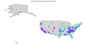
3. Implications for Policy and Research: The observed patterns emphasise the importance of understanding the underlying socio-economic, geographic, and situational factors. Such insights can guide more informed policy decisions and further research endeavours.

Introduction

The dataset provides information on fatal police shootings in the US. This report outlines the results of three machine learning classification tasks performed on the dataset: predicting the manner of death, predicting the perceived threat level, and predicting whether a body camera was active during the incident.

Task 1: Predict manner_of_death

Features used: armed, age, race, threat_level, and signs_of_mental_illness.

Accuracy: 0.94

Classification Report:
precision    recall  f1-score   support

0       0.95      0.99      0.97      1171
1       0.08      0.02      0.03        60

 

Feature Importance

 

Task 2: Predict threat_level

Features used: armed, age, gender, race, and signs_of_mental_illness.

Accuracy: 0.66

Classification Report:
precision    recall  f1-score   support

0       0.71      0.83      0.76       772
1       0.54      0.38      0.45       418
2       0.42      0.25      0.31        40

Feature Importance:

 

Task 3: Predict body_camera

Features used: armed, age, gender, race, threat_level, manner_of_death, and flee.

Accuracy: 0.80

Classification Report:
precision    recall  f1-score   support

False       0.86      0.92      0.89       961
True       0.14      0.08      0.10       160

Feature Importance:

 

Insights

1. Age consistently appears as a significant factor across all tasks. This suggests that the age of the individual involved plays a crucial role in various aspects of police encounters.
   2. The perceived threat level is influential in both predicting the manner_of_death and whether a body_camera was active. This highlights the importance of the perceived threat in police encounters.
   3. Armed status also has a notable influence across all tasks, emphasizing the role weapons play in these situations.
   4. Features like race, while not the most influential, still play a notable role in certain tasks. This may hint towards societal or systemic factors at play.
   5. The use of a body camera appears to be influenced by various factors, including the perceived threat, age, and race. This suggests that the decision to activate a body camera (or the scenarios where it’s active) may not be entirely random.

Fatal police shootings have been a point of contention and debate, particularly in the context of potential racial biases. In this blog, we’ll dive into a dataset that records such incidents to see if any patterns emerge.

Dataset Overview:

The dataset contains information on fatal police shootings, including details such as the individual’s race, age, threat level, and whether a body camera was present during the incident.

Key Findings:

1. Body Camera Presence by Race:
   • Asian and Black individuals had the highest percentages (around 20%) of incidents where body cameras were present.
   • White individuals and those of “Other” racial categories had the lowest percentages, below 12%.
2. Clustering by Race:
   • When clustering the data solely based on race, the clusters predominantly grouped incidents by specific racial groups, such as Black, White, Hispanic, Asian, and Native American.
3. Body Camera Filter’s Impact:
   • Filtering the data for incidents with body cameras and then clustering based on race revealed that the racial distribution of incidents with body cameras aligns with the overall racial distribution in the dataset.

Insights and Implications:

• The racial distribution of incidents with body cameras closely follows the overall racial distribution in the dataset. This might suggest that body camera usage is consistent across racial groups, although external factors, such as departmental policies, can influence this.
• Clustering based on race showed clear racial groupings, indicating that the dataset has a distinct racial distribution of incidents. However, determining racial bias requires a more in-depth analysis, taking into account population distributions, socio-economic factors, and other contextual data.
• While the presence or absence of body cameras doesn’t significantly alter the racial distribution of fatal police shootings, their presence can be vital for transparency, accountability, and building public trust.

Concluding Thoughts:

Data can provide valuable insights into complex issues like fatal police shootings. While our analysis offers an initial glimpse into patterns within the dataset, it’s crucial to approach the topic with a comprehensive perspective, considering all influencing factors.

Understanding potential biases in such incidents is essential for informed public discourse, creating effective policies, and ensuring justice and equity.

Introduction

In recent years, fatal police shootings have become a topic of intense debate and scrutiny. By leveraging geospatial data analysis techniques, we can gain insights into the patterns and concentrations of these incidents. In this blog post, we’ll walk through the process of clustering fatal police shooting events across the US and visualizing the results on a map.

Data Collection

Our dataset contains records of fatal police shootings in the US. For each incident, we have details such as the name of the individual, date of the incident, location (latitude and longitude), and other relevant attributes.

Objective

Our goal is to identify regions with higher concentrations of fatal police shootings. This can help stakeholders better understand the geographical distribution and potential hotspots.

Methodology

1. Data Preprocessing: We began by loading the dataset and focusing on the geographical coordinates (latitude and longitude) of each event.
2. Clustering with DBSCAN: To group these incidents based on proximity, we used the Density-Based Spatial Clustering of Applications with Noise (DBSCAN) algorithm. DBSCAN is particularly suited for geospatial clustering as it can identify clusters of various shapes and sizes.
3. Visualization: The identified clusters were then visualized on a map, with each cluster represented by a unique color.

Results

Upon visualizing the clusters, several observations were made:

1. Diverse Cluster Distributions: The clusters were spread out across the US, with some regions showing higher concentrations of incidents than others.
2. Urban Concentrations: Many of the clusters were located around major urban centers, suggesting a correlation between population density and the number of incidents.
3. Noise Data: Some data points did not belong to any specific cluster and were classified as “noise”. These are isolated incidents that don’t fit into the larger groupings.

Interpretation

The clustering results provide a visual representation of regions with higher concentrations of fatal police shootings. While urban centers naturally have a higher number of incidents due to their dense populations, the clustering approach helps identify regions with disproportionately high incidents relative to their size.

Conclusion

Geospatial clustering offers a powerful way to understand patterns in data that are otherwise hard to discern. By visualizing clusters of fatal police shootings, stakeholders can prioritize regions for further investigation or intervention. It’s essential to note that while clustering provides insights into the distribution and concentration of events, further analysis is needed to understand the underlying causes and factors contributing to these patterns

 

What’s Clustering?

Imagine you’ve dumped legos, toy cars, and action figures into a giant toy box. Now, you want to organize them. You’d naturally group similar toys together, right? That’s essentially what clustering does for data. It’s like a detective trying to group similar cases together without having any labels to guide them through it

Why K-Means?

There are many clustering methods out there, so why choose K-Means? K-Means is one of the simplest and most popular clustering techniques. It’s like trying to find centers in our candy analogy: the candies closest to a center (in terms of flavour) are grouped together. In K-Means, these centers are called “centroids”. The algorithm tries to find the best centroids such that the distance between the datapoints in a cluster and its centroid is minimised.

Digging into the Data

We dove into the police shootings data with a mission: to see if there were any hidden patterns. Using the K-Means clustering method, we grouped the data based on age, gender, race, and signs of mental illness. The outcome? Three distinct clusters:

• Cluster 0: 1583 incidents
• Cluster 1: 6014 incidents
• Cluster 2: 361 incidents

Interpreting the Clusters

• Cluster 0 (1583 incidents): Without diving deep into the data, it’s hard to give a precise interpretation. However, this could represent incidents involving a particular age group, gender, or race. It might also highlight incidents where signs of mental illness were apparent.
• Cluster 1 (6014 incidents): Being the largest cluster, this might represent the most “common” type of incident based on the features chosen. It could be incidents involving a dominant age group or gender, for instance.
• Cluster 2 (361 incidents): This being the smallest cluster could indicate rare cases or outliers. For example, it might represent incidents involving older age groups or a particular combination of features.

Potential Implications

Understanding these clusters can shed light on potential biases or patterns in police shootings. For instance, if one cluster predominantly represents a specific racial group, it could indicate a bias that needs further investigation. On the other hand, if a cluster shows a high prevalence of signs of mental illness, it could point towards the need for better mental health interventions and training for law enforcement officers.

The data on police shootings, obtained from the Washington Post, provides valuable insights into various aspects of these unfortunate events. But first lets begin by understanding some methods and what they do.

What is Logistic Regression?

Logistic regression is a statistical method for analysing datasets where the outcome variable is binary (e.g., 0/1, Yes/No, True/False). It predicts the probability that a given instance belongs to a particular category.

In our analysis of police shootings data, we used logistic regression to predict if an individual was armed based on several factors: age, gender, race, flee status, and signs of mental illness.

Logistic Regression on Predicting Armed Status: Using age, gender, race, flee status, and signs of mental illness as predictors, our model achieved an accuracy of 93%. However, it showed a strong bias towards predicting that individuals were armed, indicating that there is potential need for further refinement or balancing techniques.

Why not Linear Regression?

While linear regression predicts a continuous outcome, logistic regression predicts the probability of an event occurring. It ensures that the predicted probabilities are between 0 and 1 using the logistic function (or sigmoid function).

Results & Implications:

Our model achieved a high accuracy of 93%. However, its bias towards predicting that individuals were armed indicates a potential  imbalance.

In real-world scenarios, it’s crucial not just to consider accuracy but also other metrics like precision, recall, and the F1-score. Especially in sensitive contexts like police shootings, false negatives or false positives can have serious implications.

 

Permutation Tests: Empirical Hypothesis Testing

Permutation tests are a non-parametric method to test hypotheses. By shuffling labels and recalculating the test statistic, we can estimate a p-value based on the proportion of reshuffled datasets that provide as extreme (or more extreme) results as the original observed data.

In our analysis, the permutation test indicated a significant relationship between race and the likelihood of being armed during a police encounter.

Hypothesis Testing with Permutation Tests: We used a permutation test to examine the relationship between race and being armed. Our p-value of approximately 0.0163 suggests a significant relationship.

Predictive Analysis of Diagnosed Diabetes Prevalence_ Insights from the Center for Disease Control's Data

1. Bootstrapping:

Bootstrapping involves randomly sampling from your dataset with replacement to create many “resamples” of your data. Each resample is used to estimate the model and derive statistics. Bootstrapping provides a way to assess the variability of your model estimates, giving insight into the stability and robustness of your model.

2. Cross-Validation:

Cross-validation (CV) is a technique used to assess the predictive performance of a model. The most common form is k-fold CV, where the data is divided into $k$ subsets (or “folds”). The model is trained on folds and tested on the remaining fold. This process is repeated $k$ times, each time with a different fold as the test set. The results from all $k$ tests are then averaged to produce a single performance metric.

Combining Bootstrapping and Cross-Validation:

The combination involves performing cross-validation within each bootstrap sample. Here’s a step-by-step breakdown:

1. Bootstrap Sample: Draw a random sample with replacement from your dataset.
2. Cross-Validation on the Bootstrap Sample: Perform k-fold cross-validation on this bootstrap sample.
3. Aggregate CV Results: After the $k$ iterations of CV, average the performance metrics to get a single performance measure for this bootstrap sample.
4. Repeat: Repeat steps 1-3 for many bootstrap samples.
5. Analyze: After all bootstrap iterations, you’ll have a distribution of the cross-validation performance metric. This distribution provides insights into the variability and robustness of your model’s performance.

Why Combine Both?

1. Model Stability: By bootstrapping the data and then performing cross-validation, you can assess how sensitive the model’s performance is to different samples from the dataset. If performance varies greatly across bootstrap samples, the model might be unstable.
2. Performance Distribution: Instead of a single CV performance metric, you get a distribution, which gives a more comprehensive view of expected model performance.
3. Model Complexity: For multiple linear regression, you can assess how different combinations of predictors impact model performance across different samples. This can inform decisions about feature selection or model simplification.

Challenges:

• Computationally Intensive: This approach can be computationally demanding since you’re performing cross-validation many times depending on the size of your dataset.
• Data Requirements: You need a reasonably sized dataset. If your dataset is too small, bootstrapping might not provide meaningful variability in samples.

In conclusion, combining bootstrapping with cross-validation offers a robust method for evaluating the performance and stability of a multiple linear regression model. However, it’s essential to be aware of the computational demands and ensure that your dataset is suitable for this approach.